Table of Contents
1. Introduction: Algorithm Efficiency (and why we care)
Processing power continues increasing as time moves forward. Many things process so quickly that we barely notice it, if at all. That doesn't mean we can just write code as inefficiently as possible and just let it run because "computers are fast enough, right?" - as technology evolves, we crunch more and more data, and as "big data" becomes a bigger field, we need to work with this data efficiently - because it doesn't matter how powerful a machine is, processing large quantities of data with an inefficient algorithm can still take a long time.
And some computers today are slow. Not usually the computers that the average person is using (Even though it might feel that way if they're running Windows). Some computers that handle systems are pretty basic, or they're small, and don't have the luxury of having great specs. Fitness trackers, dedicated GPS devices, a thermostat, etc. For systems like these, processing efficiency is important.
Let's say our algorithm's time to execute increases quadratically. That means, as we increase the amount of items to process (\(n\)), the time to process that data goes up quadratically.
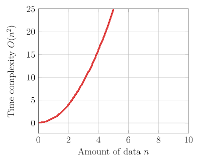
For processing 1 piece of data, it takes 1 unit of time (we aren't focused so much on the actual unit of time, since each machine runs at different speeds) - that's fine. Processing 2 pieces of data? 4 units of time. 8 pieces of data? 64 units of time. We don't just double the amount of time it takes when we double the data - we square it.
How much data do you think is generated every day on a social media website that has millions of users? Now imagine the processing time for an algorithm with a quadratic increase…
| Data to process (n) | Time to process ("time units") |
|---|---|
| 1 | 1 |
| 2 | 4 |
| 3 | 9 |
| 4 | 16 |
| 5 | 25 |
| … | … |
| 100 | 10,000 |
| 1,000 | 1,000,000 |
| 10,000 | 100,000,000 |
| 1,000,000 | 1,000,000,000,000 |
From a design standpoint we also need to know what the efficiency of different algorithms are (such as the algorithm to find data in a Linked List or the algorithm to resize a dynamic array) in order to make design decisions on what is the best option for our software.
Review 1. Some of the growth rates we care about when ti comes to computers are… (select all appropriate answers)
- □ Amount of space/memory taken up
- □ How many function calls are in the program
- □ How many user inputs are required
- □ Time to process
Example: Fibonacci sequence, iterative and recursive
As an example, you shouldn't use a recursive algorithm to generate a Fibonacci sequence (Each number \(F_n\) in the sequence is equal to the sum of the two previous items: \(F_n = F_{n-1} + F_{n-2}\)). It's just not as efficient! Let's look at generating the string of numbers:
1, 1, 2, 3, 5, 8, 13, 21, 34, 55
The most efficient way to do this would be with an iterative approach using a loop. However, we could also figure it out with a recursive approach, though the recursive approach is much less efficient.
Fibonacci sequence, iterative:
int GetFib_Iterative(int n)
{
  if (n == 0 || n == 1) { return 1; }

  int n_prev = 1;
  int n_prevprev = 1;
  int result = 0;

  for (int i = 2; i <= n; ++i)
    {
      result = n_prev + n_prevprev;
      n_prevprev = n_prev;
      n_prev = result;
    }

  return result;
}
This algorithm has a simple loop that iterates \(n\) times to find a given number of the Fibonacci sequence. The amount of time the loop iterates based on \(n\) is:
| n | 3 | 4 | 5 | 6 | 7 | 8 | 9 | 10 | … | 20 |
| iterations | 2 | 3 | 4 | 5 | 6 | 7 | 8 | 9 | … | 19 |
Fibonacci sequence, recursive:
int GetFib_Recursive(int n)
{
  if (n == 0 || n == 1) { return 1; }

  return GetFib_Recursive(n - 1) + GetFib_Recursive(n - 2);
}
The way this version is written, any time we call this function with any value \(n\), it has to compute the Fibonacci number for \(Fib(n-1)\), \(Fib(n-2)\), \(Fib(n-3)\), … \(Fib(1)\), \(Fib(0)\) … twice. This produces duplicate work b ecause it effectively doesn't "remember" what \(Fib(3)\) was after it computes it, so for \(Fib(n)\) it has to recompute \(Fib(n-1)\) and \(Fib(n-2)\) each time…
| n | 3 | 4 | 5 | 6 | 7 | 8 | 9 | 10 | … | 20 |
| iterations | 2 | 4 | 7 | 12 | 20 | 33 | 54 | 88 | … | 10,945 |
The growth rate of the iterative version ends up being linear: As \(n\) rises linearly, the amount of iterations also goes up linearly. The growth rate of the recursive function is exponential: As \(n\) rises linearly, the amount of iterations goes up exponentially.
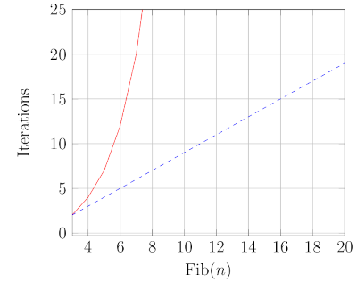
- Red/solid: Recursive growth rate
- Blue/dashed: Iterative growth rate
- Y scale from 0 to 25 (the 0th, to 25th Fibonacci number to generate).
For small amounts this might not be too bad. However, if we were generating a Fibonacci number further in the list, it would continue getting even slower…
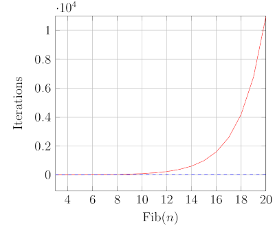
- Red/solid: Recursive growth rate
- Blue/dashed: Iterative growth rate
- Y scale from 0 to 11,000 (the 11,000th Fibonacci number to generate).
If we are trying to generate the 11,000th item in the sequence, the iterative approach requires 11,000 iterations in a loop. That linear increase is still much faster than each \(Fib(n)\) calling \(Fib(n-1)\) and \(Fib(n-2)\) recursively.
Review 2. If we model the time-growth rate for a function as \(T(n) = n^2\) then processing 6 items would result in a processing time of __ time-units.
Review 3. If we modeled the time-growth rate for a function as \(T(n) = n\) then processing 6 items would result in a processing time of __ time-units.
Review 4. Which growth rate scales better?
- ○ \(T(n) = n\)
- ○ \(T(n) = n^2\)
2. Big-O Notation and Growth Rates
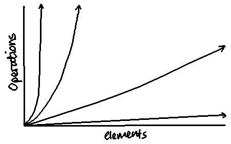
For the most part, we don't care much about the exact amount of times a loop runs. After all, while the program is running, n could be changing depending on user input, or how much data is stored, or other scenarios. Instead, we are more interested in looking at the big picture: the generalized growth rate of the algorithm. (This can include time-to-process growth or space growth.)
We use something called "Big-O notation" to indicate the growth rate of an algorithm. Some of the rates we care about are:
| Constant time | O(1) |
| Logarithmic time | O(log(n)) |
| Linear time | O(n) |
| Quadratic time | O(n2) |
| Cubic time | O(n3) |
| Exponential time | O(2n) |
2.1. Constant time, \(O(1)\)
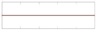
We think of any single command as being constant time. The operation a = b + c will take the same amount of computing time no matter what the values of a, b, and c are.
int F(int x)
{
  return 3 * x + 2;
}
Review 5. Let's say an algorithm's time complexity is constant. Perhaps we can model the efficiency as \(T(n) = 5\), where \(n\) is the amount of items to process and \(T\) is the time it takes.
- a. Processing 1 item would cost __ time units.
- b. Processing 10 item would cost __ time units.
- c. Processing 100 item would cost __ time units.
2.2. Logarithmic time, \(O(log(n))\)
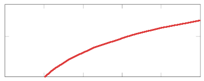
Having an algorithm that halves its range each iteration of the loop will result in a logarithmic growth rate.
int Search(int l, int r,
           int search, int arr[])
{
  while ( l <= r )
    {
      int m = l + (r-l) / 2;
      if ( arr[m] == search )
        { return m; }
      else if ( arr[m] < search )
        { l = m+1; }
      else if ( arr[m] > search )
        { r = m-1; }
    }
  return -1;
}
2.3. Linear time, \(O(n)\)
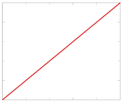
Having a single loop that iterates over a range will be a linear time increase.
int Sum( int n ) {
  int sum = 0;
  for (int i=1; i<=n; i++) {
    sum += n;
  }
  return sum;
}
If there is some scenario that causes the loop to halve its range each time, then its growth rate would be less than linear: as (log(n)).
Review 6. Let's say an algorithm's time complexity is linear. Perhaps we can model the efficiency as \(T(n) = 2n\), where \(n\) is the amount of items to process and \(T\) is the time it takes.
- a. Processing 1 item would cost __ time units.
- b. Processing 10 item would cost __ time units.
- c. Processing 100 item would cost __ time units.
2.4. Quadratic time, \(O(n^2)\)
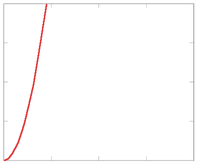
Quadratic time comes into play when you have one loop iterating n times nested within an other loop that also iterates n times. For example, if we were writing out times tables from 1 to 10 (n = 10), then we would need 10 rows and 10 columns, giving us 102 = 100 cells.
void TimesTables(int n) {
  for (int y=1; y<=n; y++) {
    for (int x=1; x<=n; x++) {
      cout << x << "*" << y << "="
           << x*y << "\t";
    }
    cout << endl;
  }
}
Review 5. Let's say an algorithm's time complexity is quadratic. Perhaps we can model the efficiency as \(T(n) = n^2\), where \(n\) is the amount of items to process and \(T\) is the time it takes.
- a. Processing 1 item would cost __ time units.
- b. Processing 10 item would cost __ time units.
- c. Processing 100 item would cost __ time units.
2.5. Cubic time, \(O(n^3)\)
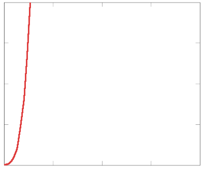
Just like nesting two loops iterating n times each gives us a n2 result, having three nested loops iterating \(n\) times each gives us a O(n3) growth rate.
void CubicThing(int n) {
  for (int z=1; z<=n; z++) {
    for (int y=1; y<=n; y++) {
      for (int x=1; x<=n; x++) {
        cout << x << " "
             << y << " "
             << z << endl;
      }
    }
  }
}
2.6. Exponential time, \(O(2^n)\)
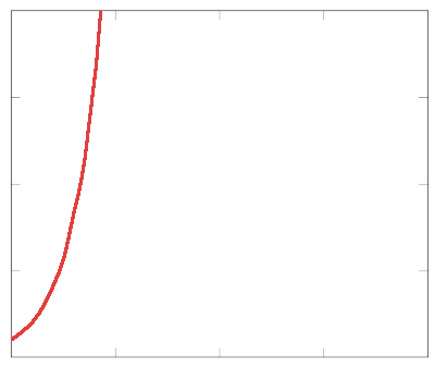
With an exponential function, each step increases the complexity
of the operation. The Fibonacci example is a good illustration:
Figuring out Fib(0) and Fib(1) are constant, but Fib(2) requires
calling Fib(0) and Fib(1), and Fib(3) calls Fib(1) and Fib(2),
with Fib(2) calling Fib(0) and Fib(1), and each iteration adds
that many more operations.
int Fib(int n)
{
  if (n == 0 || n == 1)
    return 1;

  return
    Exponential_Fib(n-2) +  Exponential_Fib(n-1);
}
3. Counting commands
We are more interested in generalizations about efficiency, but for now let's count concrete commands executed that occur with an algorithm.
We can treat a single command (like a variable assignment) as a constant 1, but once we hit a loop, the internal command is executed 1 * n times.
Let's look at how many commands are executed based on (1) the input value n, and (2) the amount of commands in the algorithm.
And note, we don't count the function header and opening/closing curly braces as a command. Only the contents of the function.
Example 1
int Func( int n )
{
  return 3 * n; // +1 command
}
How many commands are executed when…
- n = 1 ?
- n = 1 0?
- n = 100 ?
This is a constant time, so no matter what n is, we will always just be executing one arithmetic command.
Example 2
int Func( int n )
{
  n += 1; // +1 command

  if ( n > 100 )
    return n+100; // +1 command, or
  else if ( n > 10 )
    return n+10; // +1 command, or
  else
    return n; // +1 command
}
Given the if/else if statement, note that only one of these will be executed. Don't count the if/else if statement itself, just the return commands.
How many commands are executed when…
- n = 1 ?
- n = 10 ?
- n = 100 ?
This is another example of a constant time algorithm. Evaluating the "if" statements are essentially negligible, time-complexity-wise.
Example 3
void Func( int n )
{
  for ( int i = 0; i < n; i++ )
  {
    cout << i << " "; // +1 command each iteration
  }
}
How many commands are executed when…
- n = 1 ?
- n = 10 ?
- n = 100 ?
Since we have a loop in here, it runs n commands, so the amount of commands executed are affected by the n value. In this case, with just the one loop, this is a linear time increase.
Example 4
void Func( int n )
{
  int iterations = 0; // Don't count me
  for ( int i = 0; i < n; i++ )
  {
    for ( int j = 0; j < n; j++ )
    {
      cout << i << "," << j << endl; // +1 command each iteration
      iterations++; // Don't count me
    }
  }
  cout << "Iterations: " << iterations << endl; // Don't count me
}
(You can put this code in an IDE to see the result for different n
values. Just ignore the items marked // Don't count me.)
How many commands are executed when…
- n = 1 ?
- n = 10 ?
- n = 100 ?
Given some n value the nested loops will cause some command to be processed n2 amount of times. This increase is quadratic.
Review 8. Given the function:
int F(int x)
{
  return 3 * x + 2; // +1 command
}
Identify the commands-to-process for each:
- a.
F(2)is __ command(s). - b.
F(5)is __ command(s).
9. Given the function:
int Sum( int n ) {
  int sum = 0;
  for (int i=1; i<=n; i++) {
    sum += n;  // +1 command
  }
  return sum;
}
Identify the commands-to-process for each:
- a.
Sum(5)is __ command(s). - b.
Sum(10)is __ command(s).
Review 10. Given the function:
void TimesTables(int n) {
  for (int y=1; y<=n; y++) {
    for (int x=1; x<=n; x++) {
      cout << x << "*" << y << "="
           << x*y << "\t";  // +1 command
    }
    cout << endl; // (ignore for this example)
  }
}
Identify the commands-to-process for each:
- a.
TimesTables(5)is __ command(s). - b.
TimesTables(10)is __ command(s).
Review 11. Given the function:
void CubicThing(int n) {
  for (int z=1; z<=n; z++) {
    for (int y=1; y<=n; y++) {
      for (int x=1; x<=n; x++) {
        cout << x << " "
             << y << " "
             << z << endl; // +1 command
      }
    }
  }
}
Identify the commands-to-process for each:
- a.
CubicThing(5)is __ command(s). - b.
CubicThing(10)is __ command(s).
Review 12. Given the function:
int Func( int n )
{
  n += 1;             // +1 command

  if ( n > 100 )
    return n+100;    // +1 command, or
  else if ( n > 10 )
    return n+10;     // +1 command, or
  else
    return n;        // +1 command
}
With the if/else if statement, note that only one of these will be executed. Don't count the if/else if statement itself, just the return commands.
How many commands are executed for each of the following…
- a.
Func(1)is __ command(s). - b.
Func(10)is __ command(s). - c.
Func(100)is __ command(s).
Review 13. When a function doesn't contain any loops, the amount of
commands executed given an increasing n value is
○ constant / ○ a linear growth / ○ a quadratic growth
4. Identifying growth rates
We were just counting amount of commands or iterations for a function, but we aren't concerned with these concrete numbers when we are analyzing the efficiency of an algorithm. Instead, we care about generalized growth rate.
Here's a "cheat sheet" for quickly identifying algorithm increases. This is for very general cases, so you may need to study an algorithm more to figure out its actual growth rate.
| Growth rate | Big-O notation | Identification |
|---|---|---|
| Constant | O(1) | Single statements |
| Logarithmetic | O(log(n)) | Algorithm halves its work each iteration |
| Linear | O(n) | A for loop |
| Quadratic | O(n2) | Two for loops nested |
| Exponential | O(2n) | Algorithm doubles its work each iteration |
Review 14. Identify the growth rate for each given function:
a. Print function
void Print( string label, string value )
{
  cout << label << ": " << value << endl;
}
b. DrawBox function
void DrawBox( int width, int height )
{
  for ( int y = 0; y < height; y++ )
  {
    for ( int x = 0; x < width; x++ )
    {
      cout << "*";
    }
    cout << endl;
  }
}
c. DrawLine function
void DrawLine( int n )
{
  for ( int i = 0; i < n; i++ )
  {
    cout << "-";
  }
}